One thousand captcha photos organized with a neural network
Coauthored with Habib Talavati. Originally published on the Clarifai blog at https://blog.clarifai.com/one-thousand-captcha-photos-organized-with-a-neural-network-2/
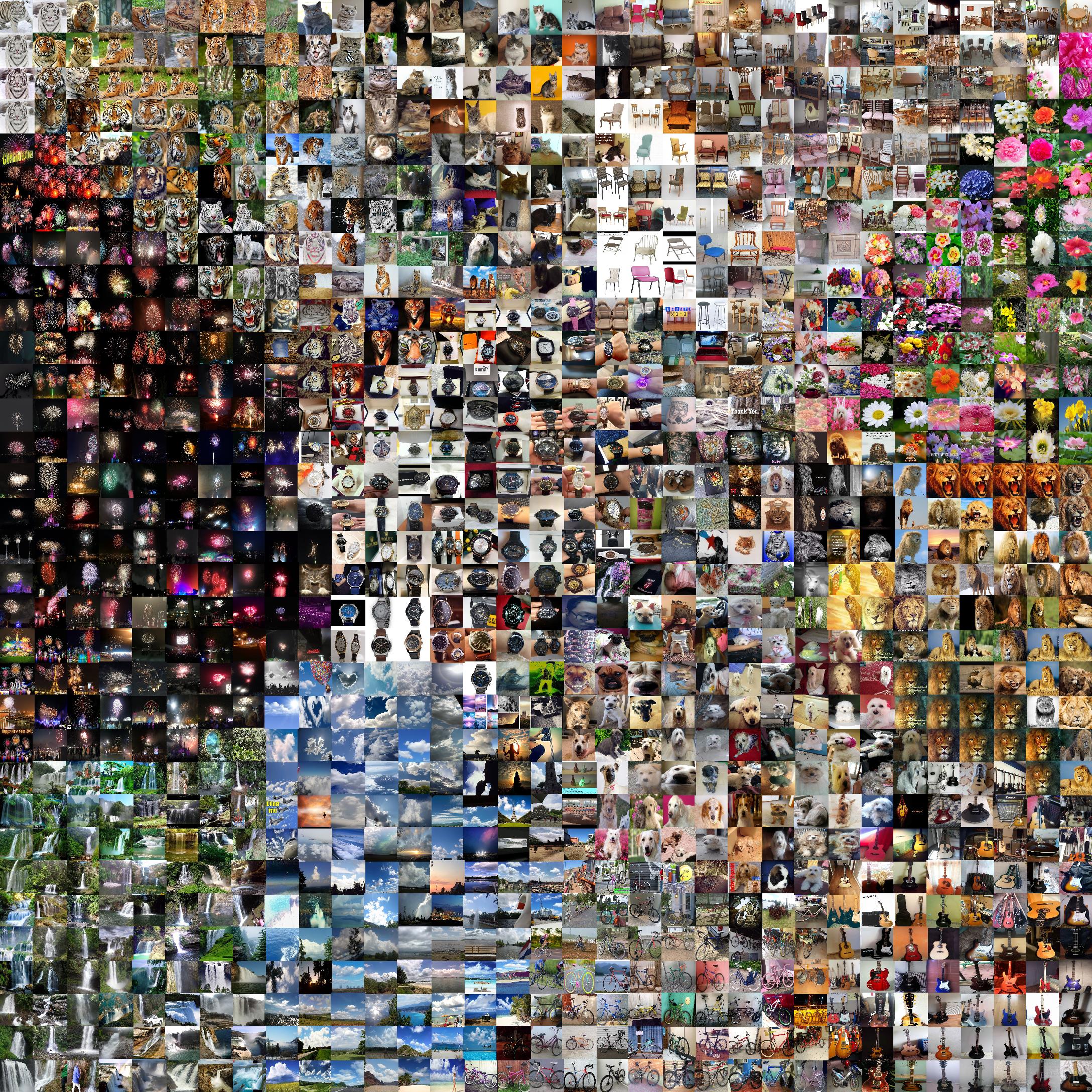
The below image shows 1024 of the captcha photos used in “I’m not a human: Breaking the Google reCAPTCHA” by Sivakorn, Polakis, and Keromytis arranged on a 32x32 grid in such a way that visually-similar photos appear in close proximity to each other on the grid.

How did we do this?
To get from the collection of captcha photos to the grid above we take three steps: embedding via a neural net, further dimension reduction via t-SNE, and finally snapping things to a grid by solving an assignment problem.
Images are naturally very high-dimensional objects, even a “small” 224x224 image requires 2242243=150,528 RGB values. When represented naively as huge vectors of pixels visually-similar images may have enormous vector distances between them. For example, a left/right flip will generate a visually-similar image but can easily lead to a situation where each pixel in the flipped version has an entirely different value from the original.
Remark: Code for all of this is available here: https://github.com/Clarifai/public-notebooks/blob/master/gridded_tsne_blog_public.ipynb

Step 1: Reducing from 150528 to 1024 dimensions with a neural net
Our photos begin as 224x224x3 arrays of RGB values. We pass each image through an existing pre-trained neural network, Clarifai’s general embedding model which provides us with the activations from one of the top layers of the net. Using the higher layers from a neural net provides us with representations of our images which are rich in semantic information - the vectors of visually similar images will be close to each other in the 1024-dimensional space.
Step 2: Reducing from 1024 to 2 dimensions with t-SNE
In order to bring things down to a space where we can start plotting, we must reduce dimensions again. We have lots of options here. Some examples:
Inductive methods for embedding learning
Techniques such as the remarkably hard-to-Google Dr. LIM or Siamese Networks with triplet losses learn a function that can embed new images to fewer dimensions without any additional retraining. These techniques perform extremely well on benchmark datasets and are a great fit for online systems which must index previously-unseen images. For our application, we only need to get a fixed set of vectors reduced to 2D in one large, slow, step.
Transductive methods for dimensionality reduction
Rather than learning a function which can new points to few dimensions we can attack our problem more directly by learning a mapping from the high-dimensional space to 2D which preserves distances in the high-dimensional space as much as possible. Several techniques are available: t-SNE, and largeVis to name a few. Other methods, such as PCA, are not optimized for distance preservation or visualization and tend to produce less interesting plots. t-SNE, even during convergence, can produce very interesting plots (cf. this demonstration by @genekogan here ).
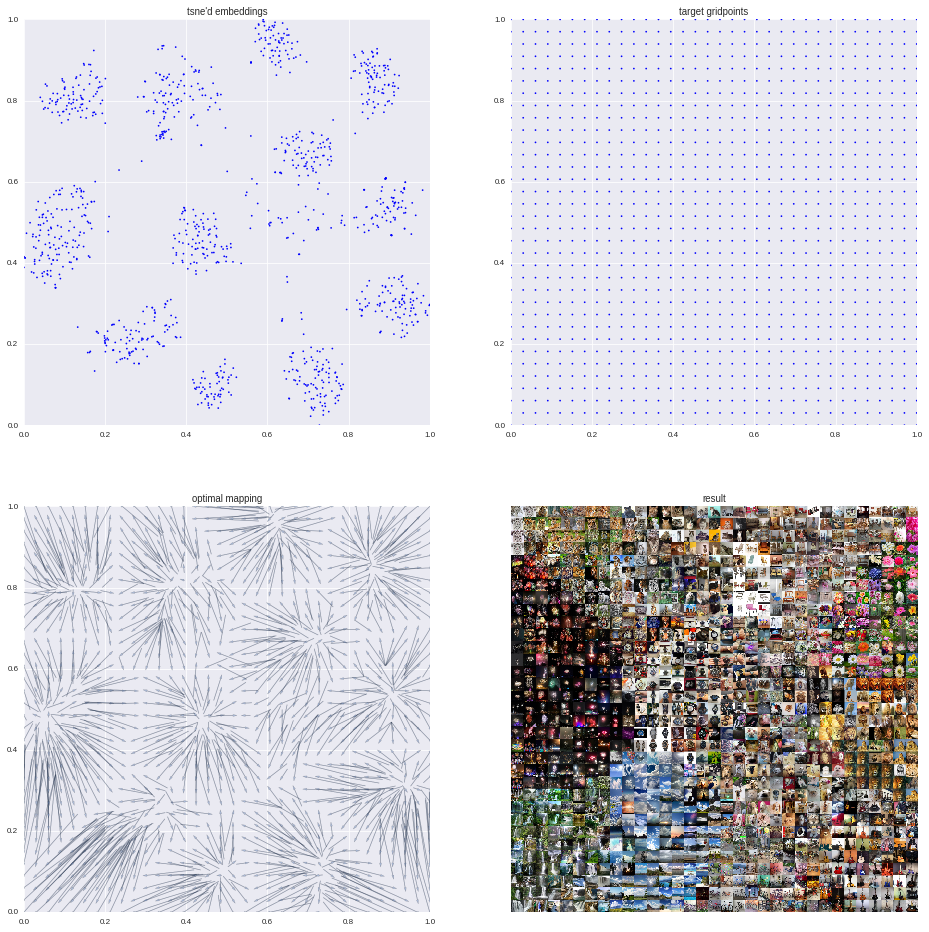
We use t-SNE to map our 1024D vectors down to 2D and generate the first entry in the above grid. Recall that our high-dimensional space here are 1024D vector embeddings from a neural net, so proximal vectors show correspond to visually similar photos. Without the neural net t-SNE would be a poor choice as distances between the initial 224x224x3 vectors are uninteresting.
Step 3: Snapping to a grid with the Jonker-Volgenant algorithm
One problem with t-SNE’d embeddings is that if we displayed the images directly over their corresponding 2D points we’d be left with swaths of empty white space and crowded regions where images overlap each other. We remedey this by building a 32x32 grid and moving the t-SNE’d points to the grid in such a way that total distance traveled is optimal.
It turns out that this operation can be incredibly sophisticated. There is an entire field of mathematics, transportation theory, concerned with solutions to problems in optimal transport under various circumstances. For example, if one’s goal is to minimize the sum of the squares of all distances traveled rather than simply the sum of the distances traveled (ie the l2 Monge-Kantorovitch mass transfer problem) an optimal mapping can be found by recasting the assignment problem as one in computational fluid dynamics and solving the corresponding PDEs. Cedric Villani, who won a Fields medal in 2010, wrote a great book on optimal transportation theory which is worth taking a look at when you get tired of corporate machine learning blogs.
In our setting, we just want the t-SNE’d points to snap to the grid in a way that makes this look visually appealing and be as simple as possible. Thus, we search for a mapping that minimizes the sum of the distances traveled via a linear assignment problem. The textbook solution here is to use the Hungarian algorithm, however, this can be also be solved quite easily and much faster using Jonker-Volgenant and open source tools
How easy can we make this?
Pretty easy. In addition to the notebook listed above, we’ve also set up an API endpoint that will generate an image similar to the one above for an existing Clarifai application. Here we assume you already have created an application by visiting https://developer.clarifai.com/account/applications and added your favorite images to it by calling the resource https://api.clarifai.com/v2/inputs. Then all you have to do is this:
Step 1: Kick off an asynchronous gridded t-SNE visualization
Since generating a visualization takes a while, we generate one asynchronously. We kick off a visualization by calling
POST https://api.clarifai.com/v2/visualizations/
You should get a response like below informing us a “pending” visualization is scheduled to be computed
{
    "output": {
        "id": "ca69f34d53c742e1b4a1b71d7b4b4586",
        ...
    }
}
Note the id ca69f34d53c742e1b4a1b71d7b4b4586. We will use that id to get the visualization we just kicked off.
Step 2: Check to see if the visualization is done
Call GET /v2/visualizations/ca69f34d53c742e1b4a1b71d7b4b4586. The returned visualization will be “pending” for a while, but eventually, we should get a response like this:
{
    "output": {
        "data": {
            "image": {
                "url": "https://s3.amazonaws.com/clarifai-visualization/gridded-tsne/staging/your-visualization.jpg"
            }
        },
        ...
    }
}
At last, the output.data.image.url contains your gridded t-SNE visualization.