Darknet Market Basket Analysis
The Evolution darknet marketplace was an online black market which operated from January 2014 until Wednesday of last week when it suddenly disappeared. A few days later, in a reddit post, gwern released a torrent containing daily wget crawls of the site dating back to its inception. I ran some off-the-shelf affinity analysis on the dataset – here’s what I found:
Products can be categorized based on who sells them
On Evolution there are a few top-level categories (“Drugs”, “Digital Goods”, “Fraud Related” etc.) which are subdivided into product-specific pages. Each page contains several listings by various vendors.
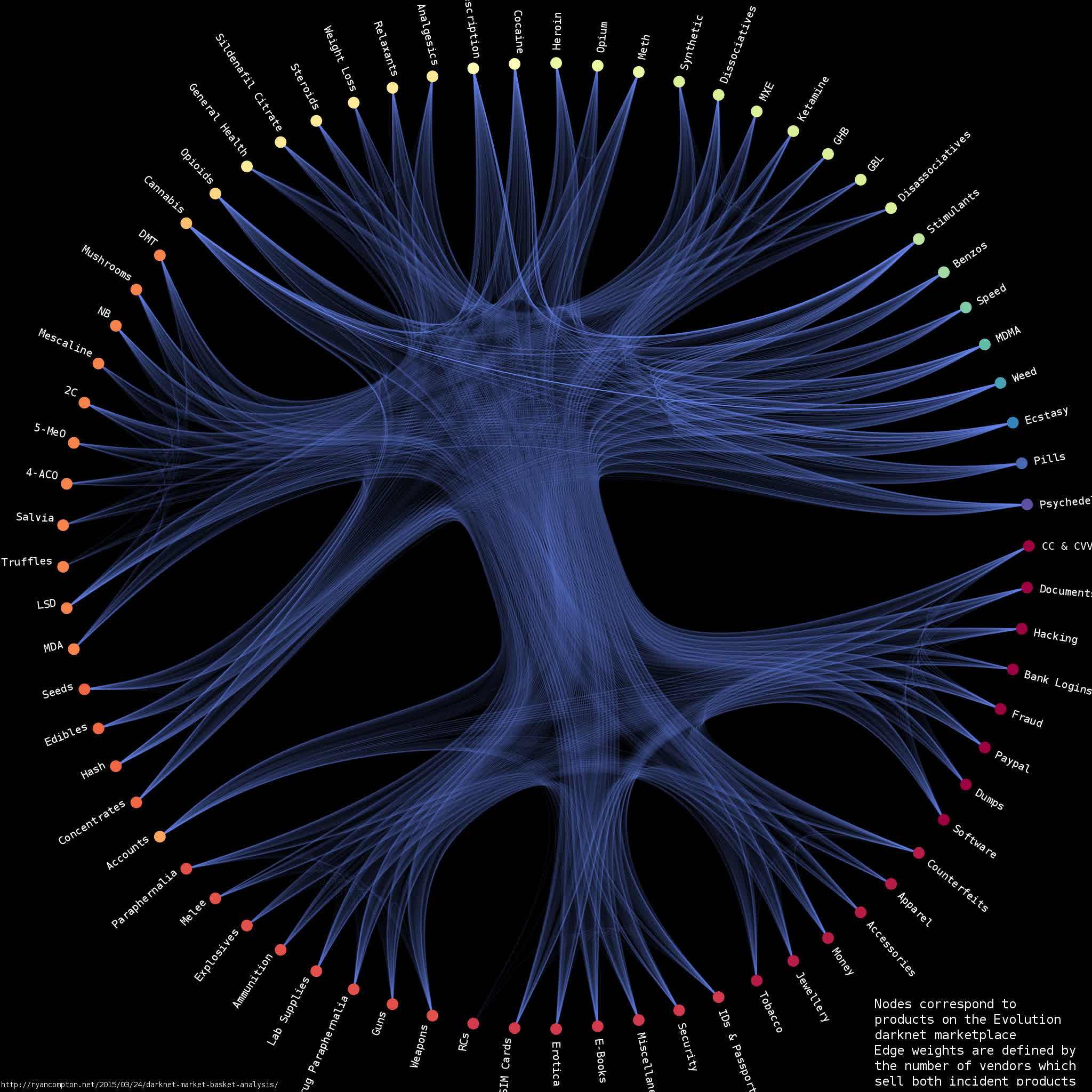
I built a graph between products based on vendor co-occurrence relationships, i.e. each node corresponds to a product with edge weights defined by the number of vendors who sell both incident products. So, for example, if there are 3 vendors selling both mescaline and 4-AcO-DMT then my graph has an edge with weight 3 between the mescaline and 4-AcO-DMT nodes. I used graph-tool’s implementation of stochastic block model-based hierarchal edge bundling to generate the below visualization of the Evolution product network:
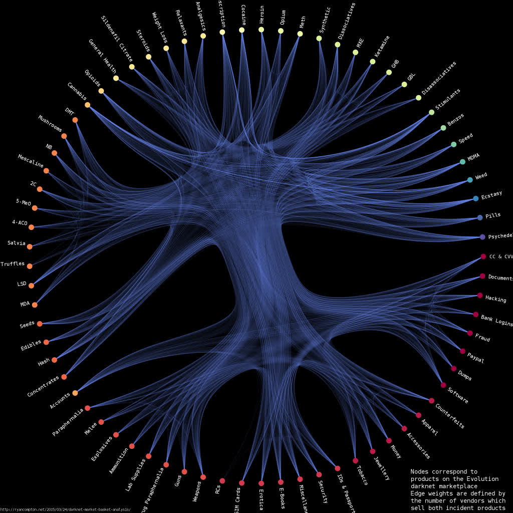
The graph is available in graphml format here. It contains 73 nodes and 2,219 edges (I found a total of 3,785 vendors in the data).
Edges with higher weights are drawn more brightly. Nodes are clustered with a stochastic block model and nodes within the same cluster are assigned the same color. There is a clear division between the clusters on the top half of the graph (correpsonding to drugs) and the clusters on the bottom half (corresponding to non-drugs, i.e. weapons/hacking/credit cards/etc.). This suggests that vendors who sold drugs were not as likely to sell non-drugs and vice versa.
I used a short python script to parse the scraped html and remove duplicate data, its available here. It takes a while to go through the entire dataset (which is about 90GB); if you’d like to skip that you can download the results of my parse as a .tsv file. The plotting code is available as an ipython notebook. High-res version of the above plot here.
91.7% of vendors who sold speed and MDMA also sold ecstasy
Association rule learning is a straightforward and popular way to solve problems in market basket analysis. The traditional application is to suggest items to shoppers based on what other customers are putting in their carts. For some reason the canonical example is “customers who buy diapers also buy beer”.
We don’t have customer data from a crawl of the public postings on Evolution. However, we do have data on what each vendor sells which can help us quantify results suggested by the visual analysis done above.
Here’s an example of what our database looks like (the complete file has 3,785 rows (one for each vendor)):
| Vendor | Products |
|---|---|
| MrHolland | [‘Cocaine’, ‘Cannabis’, ‘Stimulants’, ‘Hash’] |
| Packstation24 | [‘Accounts’, ‘Benzos’, ‘IDs & Passports’, ‘SIM Cards’, ‘Fraud’] |
| Spinifex | [‘Benzos’, ‘Cannabis’, ‘Cocaine’, ‘Stimulants’, ‘Prescription’, ‘Sildenafil Citrate’] |
| OzVendor | [‘Software’, ‘Erotica’, ‘Dumps’, ‘E-Books’, ‘Fraud’] |
| OzzyDealsDirect | [‘Cannabis’, ‘Seeds’, ‘MDMA’, ‘Weed’] |
| TatyThai | [‘Accounts’, ‘Documents & Data’, ‘IDs & Passports’, ‘Paypal’, ‘CC & CVV’] |
| PEA_King | [‘Mescaline’, ‘Stimulants’, ‘Meth’, ‘Psychedelics’] |
| PROAMFETAMINE | [‘MDMA’, ‘Speed’, ‘Stimulants’, ‘Ecstasy’, ‘Pills’] |
| ParrotFish | [‘Weight Loss’, ‘Stimulants’, ‘Prescription’, ‘Ecstasy’] |
Before saying anything more about association rule learning here’s a quick glossary of terms:
- The support, $supp(X)$, of an itemset, $X$, is defined as the proportion of transactions in the data set which contain $X$. In the table above, the support of ‘Cocaine’ is 2 because it appears in two vendors’ storefronts (MrHolland and Spinifex)
- The confidence of a rule is defined $\mathrm{conf}(X \Rightarrow Y) = \mathrm{supp}(X \cup Y) / \mathrm{supp}(X)$. In our example the confidence of the rule ‘Cannabis’ ==> ‘Cocaine’ is 2/3 because out the 3 vendors who sell ‘Cannabis’ 2 of them sell ‘Cocaine’. The support of this rule is 2.
Association rule mining is a huge field within computer science – hundreds (thousands?) of papers have been published over the past two decades. The necessary algorithms are very complex but open source implementations are available. My favorite collection (and the one I used for these experiments) is Philippe Fournier Viger’s spmf.
I ran the FP-Growth algorithm with a minimum allowable support of 40 and a minimum allowable confidence of 0.1. The algorithm learned 12,364 rules. These can be downloaded as a .tsv here. I’ve selected a few rules for display below:
| antecedent | consequent | support | confidence |
|---|---|---|---|
| [‘Speed’, ‘MDMA’] | [‘Ecstasy’] | 155 | 0.91716 |
| [‘Ecstasy’, ‘Stimulants’] | [‘MDMA’] | 310 | 0.768 |
| [‘Speed’, ‘Weed’, ‘Stimulants’] | [‘Cannabis’, ‘Ecstasy’] | 68 | 0.623 |
| [‘Fraud’, ‘Hacking’] | [‘Accounts’] | 53 | 0.623 |
| [‘Fraud’, ‘CC & CVV’, ‘Accounts’] | [‘Paypal’] | 43 | 0.492 |
| [‘Documents & Data’] | [‘Accounts’] | 139 | 0.492 |
| [‘Guns’] | [‘Weapons’] | 72 | 0.98 |
| [‘Weapons’] | [‘Guns’] | 72 | 0.40 |
Other Remarks
I think I’ve only scratched the surface of what’s possible with this data. There are much more detailed product descriptions for each listing in the .tsv. That text is harder to work with so it will take some time to figure out what makes sense.